№ 061 · Deep Dive · · 10 min
Why Market Timing Models Look Great in Backtests and Fail in Production
Learn why timing models shine in backtests and stumble with real money, and how to use trend signals without fooling yourself. See what holds up.

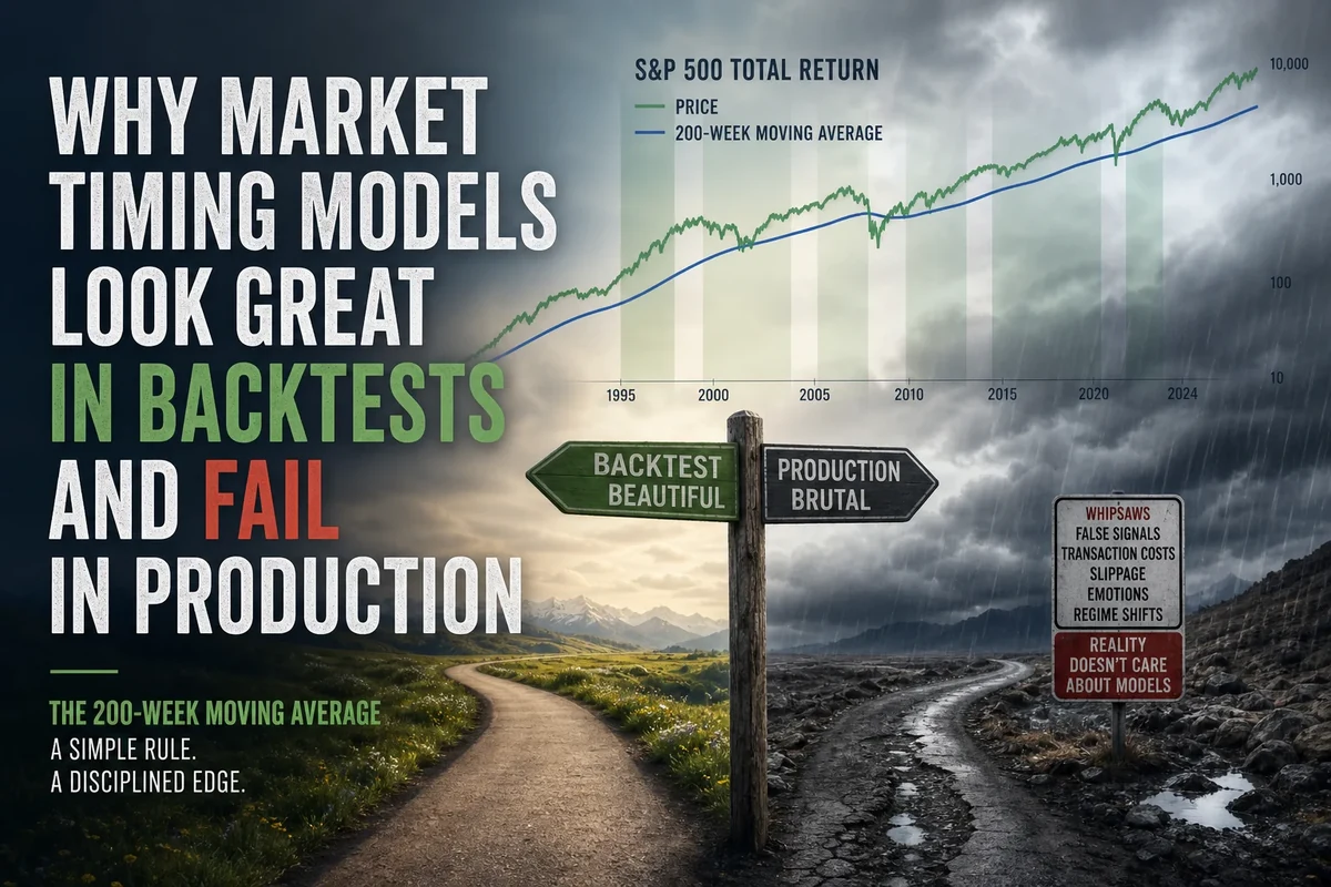
Market timing models look excellent in backtests and disappoint in production for four reasons. The rules were tuned on the same history used to grade them, trading costs and execution delays were ignored or understated, the market regime that produced the result changed, and the human running the model abandoned it during the drawdown it was built to survive. Slow trend-following rules on broad asset classes retain some real value, mainly as a way to reduce drawdown, but the live edge is almost always smaller than the backtest. Treat any simulated result as an upper bound, not a forecast.
This article draws on verified S&P 500 drawdown data, live index readings as of late September 2026, and published research on data mining and post-publication decay.
Why Do Market Timing Backtests Fail in Live Trading?
Backtests fail live largely because they fit a single historical path that will not repeat exactly. A researcher who tries enough combinations of lookback windows, asset classes, and entry rules will find some that would have worked beautifully by chance. The surviving rule gets published or sold, and the failures stay in a drawer.
A model with few parameters, tested across other markets and eras, deserves more trust than one tuned to a single index. Even then, the backtest ignores the frictions that arrive once real money is involved, and a timing edge that looks large on paper is often small enough for those frictions to consume it.
A backtest answers the question of what would have worked. Live trading asks what will work, and only rules with a durable economic reason behind them carry over from one to the other.
Overfitting Is the Invisible Tax
Data mining is among the most damaging flaws because the final chart hides it. Research on quantitative investing has repeatedly warned that we typically see only the backtests that worked. If researchers run hundreds of tests, some will show high returns by luck alone, and nothing suggests those strategies will work in the future. Cam Harvey has called this p-hacking.
The most dangerous variant uses a backtest to improve a backtest. Adjusting a moving average from 190 days to 210 days because the equity curve improves feels like refinement, yet it converts noise into apparent skill. The simpler the model, the more useful the result, and out-of-sample checks on other countries, eras, and markets are the best available defence.
Publication itself seems to degrade results. McLean and Pontiff, in their study of published equity anomalies titled Does Academic Research Destroy Stock Return Predictability?, found that returns on published strategies fell materially after publication relative to the in-sample figures. Part of that decline reflects statistical bias in the original result, and part reflects investors arbitraging the pattern away.
A thought experiment from quantitative research makes the behavioural side vivid. Imagine three managers handed the formulas for eight popular factors in 1977, plus proof that all of them would be profitable over the next 39 years. The manager who equal-weighted all eight earned about 2.4% a year in alpha. The manager who chased the recent best performers earned about 1.2%, and the manager who favoured the recent worst performers earned about 3.3%. Even with perfect knowledge that every idea works, tactical switching toward recent winners cut the return by half.
Costs, Delay, and Taxes Erode a Thin Edge
Backtests typically assume you trade at the close of the day the signal fires. In practice you learn the signal after the close and trade the next morning, or the next month. A more useful test is to delay the signal and see what survives. A study of momentum-based allocation across equities, bonds, gold, and cash, published as Part 63 of the Safe Withdrawal Rate series, did exactly that. Delaying the signal by a full month cut the Sharpe ratio by roughly 0.07 to 0.09 while leaving drawdowns about the same. That is a modest penalty for a slow monthly rule, and a faster signal would likely suffer more.
Transaction costs scale with turnover. A strategy that switches rarely pays little, while one that flips every few weeks pays spreads, commissions, and market impact each time. A commenter in a discussion of fundamental indexing put the arithmetic plainly. If a strategy adds 2% of alpha a year in theory but costs 2% more to implement, the alpha disappears. In a good year the strategy might add 8% and still show 6% after costs, but in a mediocre year a 1% gain becomes a 1% loss.
Taxes rarely appear in backtests. Exiting a long-held equity position to sit in cash crystallises gains that a buy-and-hold investor defers for decades, so a timing model in a taxable account has to clear a considerably higher hurdle.
Regime Change and the Crowding Problem
Even a rule that is honestly discovered and cheaply executed can fail when the environment shifts. The Safe Withdrawal Rate study found that most of the momentum strategy’s outperformance over a fixed 70/20/10/0 allocation occurred between 1871 and about 1940, and that the path was much smoother after World War II. It also reported worse drawdowns for the momentum strategy in the 1940s. A rule built on the persistence of economic regimes performs well when regimes persist, and less well when they do not.
Crowding adds a second layer. If timing worked easily, everyone would do it and it would stop working. Trend-following has survived for a long time, plausibly because it is uncomfortable to follow and pays off as insurance against rare crashes. Still, the more widely a specific signal is followed, the more crowded its entries and exits can become, and the worse the fills in fast markets.
The Behavioural Layer No Backtest Simulates
A major leak is the investor. A backtest executes every signal without hesitation, including the ones that feel terrible. A human being sells after a large decline, watches the market rebound, and finds it very hard to buy back at higher prices. Loss aversion is strong enough that investors often miss bull markets because of fear and panic during sell-offs, and the whipsaw that follows damages both returns and confidence.
Consider how differently the major S&P 500 bear markets unfolded. The table below uses hand-verified figures for each since 1973, as of September 2026.
| Bear market | Peak-to-trough decline | Weeks to bottom | Weeks to full recovery |
|---|---|---|---|
| 1973-74 (oil shock, stagflation) | -48% | 93 | 374 |
| 1987 (Black Monday) | -34% | 14 | 98 |
| Dot-com crash | -49% | 135 | 384 |
| Global financial crisis | -57% | 73 | 207 |
| COVID crash | -34% | 5 | 21 |
| 2022 bear | -25% | 40 | 68 |
In the slow declines of 1973, 2000, and 2008, a trend rule had many weeks to act and could have reduced the damage. In the COVID crash the market bottomed in five weeks and fully recovered in 21, so a monthly signal could easily have sold near the low and bought back well above it. No single timing model suits all six episodes, and the investor has to live through whichever type arrives next.
The hardest part of a tactical model is holding it through the stretch when it lags a simple index fund. A rule you abandon after three years of underperformance delivers the cost of the strategy and none of the benefit.
What the Evidence Supports
Simple trend filters applied to broad asset classes have a long record as drawdown reducers. Over 1995 to 2025, the Safe Withdrawal Rate study’s momentum strategy, using equities, intermediate bonds, gold, and cash, earned returns within about 100 basis points of equities a year with almost half the risk, and a nominal Sharpe ratio of about 0.95. That is a respectable result, and it held up reasonably well when the signal was delayed. It remains a simulation by a careful researcher who has since published it, which is exactly the situation where the lessons above apply.
Live experience is messier. One reader of that series reported implementing a top-three momentum approach in a retirement account at the end of 2018. Tracking from September 2018, the portfolio returned 12.14% a year with 12.59% volatility and a maximum drawdown of 8.97%, against 15.31% a year with 21.41% volatility for the S&P 500 fund SPY. The reader noted the comparison was imperfect because the strategy was built around a 60/40 portfolio. The live investor got a much smoother ride and paid for it with lower returns during a long equity bull market, a fair outcome for a risk-reduction tool and a disappointing one for anyone who bought it as a return enhancer.
A reasonable reading is that trend rules can shorten the time spent in deep drawdowns at the cost of trailing a bull market. That suits retirees worried about sequence-of-returns risk and suits a 30-year-old accumulating for decades less well.
Does the 200-Week SMA Hold Up as a Timing Tool?
Better than most, though it works best as a filter for deploying new capital rather than as a trigger to sell and rebuy. It has one parameter, it signals rarely, and it targets multi-year extremes, which keeps costs and whipsaw low. Our explainer on the 200-week SMA and the S&P 500 200-week SMA history document how often major lows have clustered near that line, and why the 200-week SMA catches what the 200-day misses compares it with shorter averages.
The limits are real. Because the signal fires infrequently, its statistical record is thin, and price has touched or briefly undercut the average at cycle lows without always stopping there. As of late September 2026, the S&P 500 stood near 7,714, about 36% above its computed 200-week SMA of roughly 5,686, a reading that offers no buy signal. The Shiller CAPE was about 41 on the same date against a long-run mean of roughly 16 to 17, yet valuation is a poor short-term timer, as we discuss in why valuation shapes the next decade without timing it.
A sober use treats the signal as a prompt to deploy new cash more aggressively when price approaches the average while leaving the core allocation in place, the approach described in the Buy the 200 strategy guide. Nothing is sold, so there is no tax drag, no whipsaw, and no buy-back decision. It gives up protection against a long decline in exchange for surviving the human factor, a trade that suits many investors.
Before trusting any timing model, check how many parameters it has and whether they were tuned on the data used to grade it. Check whether it survives a delayed signal, realistic costs, and taxes, and whether it holds on other markets and earlier periods. Then ask whether you would keep following it through three years of lagging a plain index fund. If the answer is no, the model will likely fail in your hands however good the backtest looks.
Frequently Asked Questions
Q: Why do backtests overstate market timing performance?
A: Rules are usually tuned on the same history used to evaluate them, so noise gets mistaken for skill. Backtests also assume perfect execution at the signal price, with no delay, costs, or taxes, which live trading cannot match.
Q: Does tactical asset allocation beat buy and hold?
A: Simple trend-following models have reduced drawdowns and volatility in long historical tests, and one study found returns within about 100 basis points of equities with almost half the risk from 1995 to 2025. Beating buy and hold on raw returns is much less reliable, especially after costs and taxes.
Q: Is the 200-week SMA a good market timing tool?
A: It works better as a long-cycle filter for deploying new capital than as a trigger to sell and rebuy. It signals rarely, has one parameter, and has clustered near major cycle lows, but its record rests on a small number of events.
Q: How can I tell if a timing model is overfit?
A: Overfit models typically have many parameters, were refined repeatedly against the same data, and weaken when tested on other markets or earlier periods. A rule with a clear economic rationale that survives a delayed signal and realistic costs deserves more trust.