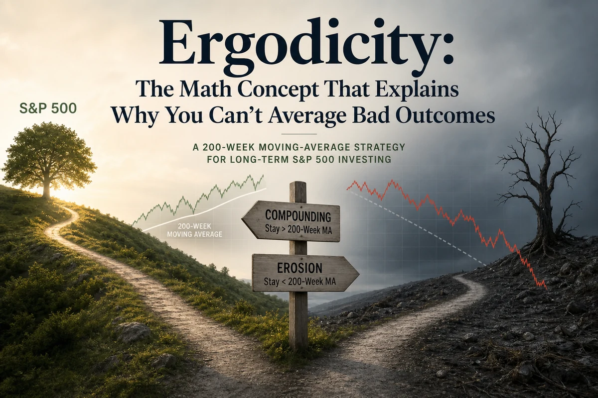
Ergodicity: The Math Concept That Explains Why You Can’t Average Bad Outcomes

Most return statistics are computed the wrong way for the question you are actually asking. A fund reports its “average annual return.” A backtesting tool shows “expected value.” A financial planner projects a smooth 7% compounding line into your retirement. Every one of these figures is technically correct and practically misleading, because they measure outcomes across a population of investors rather than through time for a single investor. That distinction is not a rounding error. It is, depending on your leverage and withdrawal rate, the difference between building wealth and losing everything while the average looks fine.

The concept that formalises this gap is ergodicity, and once you understand it, a surprisingly large number of standard investment frameworks start to look inadequate.

What Ergodicity Actually Means

A system is ergodic if the average outcome across many parallel instances equals the average outcome across one instance over a long stretch of time. Toss a fair coin one million times, and your long-run frequency of heads converges on the population average. The time-average and the ensemble-average are the same thing. That is ergodicity.

Financial returns are not ergodic. The reason is multiplicative compounding. When returns compound, the sequence in which they arrive permanently shapes the terminal outcome. A single catastrophic loss early in the series cannot be undone by averaging in better results later. The wealth path of one investor over forty years is not the same thing as the average wealth path of forty thousand investors over one year each.

When a financial model reports an “expected return,” it is computing what happens on average across all possible investors. But you are not a statistical average. You are one person, living through one sequence of returns, with a portfolio that can be permanently impaired.

This is the core of what the physicist Ole Peters and colleagues at the London Mathematical Laboratory have argued in recent years: most of neoclassical economics assumes ergodicity where none exists, and this assumption quietly distorts nearly every recommendation that follows from it.

The Arithmetic vs. Geometric Mean Problem

The clearest entry point into ergodicity is the relationship between arithmetic and geometric returns. Suppose an investment gains 50% in year one and loses 33.3% in year two. The arithmetic average return is a respectable-looking 8.35% per year. The geometric mean is exactly zero. Your ending wealth is identical to your starting wealth.

Now suppose the swings are more violent: up 100% in year one, down 50% in year two. The arithmetic average is 25% annually. The geometric mean is again zero. You have not made a cent in two years despite the headline average showing strong performance.

The formula that connects these two measures is sometimes called the volatility drag: the geometric mean approximately equals the arithmetic mean minus half the variance of returns. A portfolio with a 10% arithmetic mean and 20% annual standard deviation has a geometric mean of roughly 8% (10% minus half of 4%). A portfolio with the same arithmetic mean but a 40% standard deviation has a geometric mean closer to 2%. The drag is quadratic in volatility, which means it accelerates fast as swings get larger.

This is not a theoretical nicety. It is the mechanism by which high-volatility strategies destroy compounding wealth even when their average return looks competitive. The arithmetic mean is the figure you see in a fund factsheet. The geometric mean is what lands in your account. Over decades, the gap between them compounds into a material difference in terminal wealth.

Path Dependency and the Ruin Problem

Ergodicity becomes most dangerous at the boundary where outcomes are irreversible. Loss of capital beyond a certain threshold is not a setback you average your way out of. It is a permanent exit from the compounding game.

Consider the canonical example used in probability theory. A gambler starts with $100 and bets a fixed fraction of their wealth on a coin flip with a 60% win rate. The expected value at each flip is positive. The arithmetic mean return is positive. Yet if the fraction bet is large enough, the gambler will almost certainly go broke over a long enough horizon, because the multiplicative nature of sequential losses creates a downward absorbing barrier. Once you hit zero, you cannot recover, regardless of what the expected value says about the average outcome across all parallel gamblers.

Real investing contains the same structure. A 50% drawdown requires a 100% subsequent gain just to return to even. A 75% drawdown requires a 300% gain. These are not symmetric. The deeper the loss, the more future growth is consumed simply by getting back to the starting line, rather than advancing beyond it. Meanwhile, another investor who avoided the drawdown has been compounding the entire time. The gap between them widens not because of differential skill, but because of differential path.

Survival is not just a nice outcome. In a non-ergodic system, survival is the prerequisite for all other outcomes. An investor who avoids ruin will eventually compound. An investor who does not has no future returns to average.

This is why the body of serious financial writing, from the Kelly Criterion to modern sequence-of-returns analysis, converges on one underlying principle: the goal is not to maximise the arithmetic expected return. The goal is to maximise the long-run geometric mean while keeping the probability of ruin near zero. These two objectives are not the same, and strategies optimised for one often perform badly on the other.

Why Leverage Deserves Particular Caution

Leverage is the mechanism that most aggressively exploits the non-ergodic structure of returns. By amplifying both gains and losses, leverage widens the variance and therefore deepens the volatility drag. A 2x leveraged portfolio on an index with 20% annual standard deviation faces an effective standard deviation of 40%. The volatility drag on the leveraged position is four times larger in absolute terms. If the underlying index’s arithmetic mean is 10% and geometric mean is 8%, the 2x product’s arithmetic mean is approximately 20%, but the geometric mean might be only 12%, not 16% as naive doubling would imply.

That gap widens further when leverage introduces the possibility of a margin call or forced liquidation. At the moment the price falls far enough, the leveraged investor is compelled to sell, converting a paper loss into a permanent one. This is a hard, irreversible exit from the compounding series, exactly the ruin scenario that ergodicity analysis identifies as catastrophic. The subsequent recovery in the underlying asset is irrelevant because the investor no longer holds it.

This explains why the Kelly Criterion, a framework developed in information theory and later applied to gambling and investment sizing, recommends position sizes that are much smaller than naive expected-value maximisation would suggest. The full Kelly fraction maximises the long-run geometric mean. Fractions above it reduce the geometric mean even though they raise the arithmetic mean. Serious practitioners frequently use half-Kelly or quarter-Kelly allocations, accepting lower expected returns in exchange for a substantially reduced probability of catastrophic drawdown.

For the kind of long-term passive investor this site is written for, the practical implication is straightforward. Leveraged ETFs, margin accounts, and concentrated levered positions are products that look attractive through an arithmetic lens and are frequently destructive through a geometric one. The marketing materials for a 2x or 3x product typically show the arithmetic gain on up days. They do not show the geometric drag that accumulates quietly over years of two-sided volatility.

What This Means for Position Sizing and Diversification

If volatility drag is the mechanism, then reducing variance is not merely a comfort measure. It is a direct lever on geometric returns. A diversified portfolio that holds many uncorrelated positions instead of a handful does not just smooth the ride. It demonstrably raises the geometric mean return by compressing the variance, even if the arithmetic mean of the constituent positions is unchanged.

This gives diversification a stronger justification than the conventional “don’t put all your eggs in one basket” framing. The conventional argument is about avoiding idiosyncratic catastrophe. The ergodicity argument is subtly different and more powerful: even if you expect all your concentrated positions to perform well, combining them reduces variance and therefore raises the geometric mean that actually compounds into your terminal wealth. You can expect to be better off in a mathematical sense, not just a risk-adjusted one.

The same logic applies to volatility more broadly. Two portfolios with identical arithmetic means but different volatilities will produce different terminal wealth. The lower-volatility portfolio will compound to a higher value over time, purely as a result of arithmetic. This is not hidden in any unusual assumption. It follows directly from the formula connecting geometric and arithmetic returns. Evidence in financial research consistently shows that lower-volatility equity strategies have historically delivered competitive or superior long-run geometric returns to higher-volatility alternatives, despite appearing less exciting in any individual year.

Position sizing that ignores this will over-allocate to high-variance ideas and under-allocate to steady compounders, producing worse outcomes than the raw expected return calculation suggests. A smaller position in a volatile asset can compound to a larger terminal value than a larger position in the same asset, if the smaller size keeps the overall portfolio variance low enough to protect the geometric mean. This is counterintuitive until you have seen the numbers, and it is one of the more practically important insights ergodicity brings to everyday portfolio construction.

The Connection to Sequence Risk and the 200-Week SMA

Sequence-of-returns risk is ergodicity applied to the specific problem of withdrawals. An accumulator’s portfolio is largely indifferent to return sequence because no capital is removed. The geometric mean of the full series is determined only by the product of all the period returns, not their order. But a retiree withdrawing capital each period faces a non-ergodic trap: a bad sequence early in retirement forces asset sales at low prices, permanently reducing the base that future returns compound on. The same underlying arithmetic that makes volatility drag dangerous in accumulation makes early drawdowns catastrophic in decumulation.

Long-cycle technical tools like the 200-week simple moving average are, from an ergodicity perspective, instruments for managing path dependency rather than for predicting market direction. When the S&P 500 trades significantly above its 200-week SMA, as it does at current market levels with price roughly 41% above that long-run average, the range of potential short-term outcomes widens. A wider range of outcomes means higher effective variance, and higher variance means a larger drag on geometric returns for anyone exposed at full position through that period.

This does not require a view on whether the market will fall. It requires only an acknowledgement that the distribution of outcomes is wider at higher valuations and higher distances from long-cycle trend, and that wider distributions compound more slowly than narrow ones at equivalent arithmetic means. The disciplined approach described in the Buy the 200 strategy is, in structural terms, an ergodicity-aware framework: it increases exposure when variance is historically compressed near long-cycle support, and reduces aggressive sizing when the distribution of outcomes has widened. This is geometric-mean-maximising behaviour even if it is not described in those terms.

Managing position size based on where you are in a long market cycle is not about predicting corrections. It is about recognising that volatility drag is not constant through a cycle, and that the geometric mean cost of full exposure is highest when the variance of near-term outcomes is greatest.

Practical Rules an Ergodicity-Aware Investor Follows

Bringing this down to daily portfolio decisions, ergodicity awareness changes a few specific behaviours. First, it shifts the primary objective from maximising expected return to maximising long-run geometric mean. These sound similar. In practice, the difference shows up in how much weight you give to large downside scenarios. An expected-value maximiser treats a 10% chance of losing 80% as arithmetically offset by a 90% chance of gaining 20%. A geometric-mean maximiser recognises that the 80% loss scenario may involve ruin, and weights it severely rather than proportionally.

Second, it changes how you think about leverage and concentration. Leverage amplifies variance, which amplifies volatility drag, which reduces the geometric mean. Concentration in a single position increases idiosyncratic variance even if the expected return on that position is high. In both cases, the ergodicity-aware investor asks not “what is my expected return?” but “what volatility drag am I accepting, and does the potential gain justify the geometric-mean cost?” For many leveraged or concentrated positions, the answer is often no.

Third, it reframes diversification as a geometric return engine rather than merely a defensive measure. Adding low-correlation assets to a portfolio, even those with lower individual arithmetic returns, can raise the portfolio’s geometric mean by reducing overall variance. This is the mathematical basis for rebalancing as a return enhancer: by periodically selling appreciated assets and buying laggards, you reduce portfolio variance and therefore improve compounding. Research on rebalanced diversified portfolios consistently shows this effect, and it is entirely explicable through the volatility drag formula rather than through any claim about market timing.

Finally, it reinstates survival as a primary investment objective rather than a secondary one. An investor who never experiences permanent capital impairment will eventually accumulate significant wealth through compounding, even with modest returns. An investor who earns higher arithmetic returns but periodically suffers severe drawdowns may end up with less, because each recovery cycle is increasingly burdened by the accumulated cost of past losses. In an ergodic world, the average is a guide. In the world you actually invest in, the path is everything.

Frequently Asked Questions

Q: If the geometric mean is what matters, why do financial products advertise arithmetic returns?

A: Arithmetic returns are higher, simpler to compute, and easier to compare over short periods. They are also the legally required disclosure in most jurisdictions. The gap between arithmetic and geometric return only becomes visible over long horizons, and by then you are locked into the product. Awareness of this gap is one of the most practical things a long-term investor can carry into every performance comparison they read.

Q: Does ergodicity mean you should never use leverage?

A: Not categorically. Small amounts of leverage applied conservatively, well below the Kelly optimal fraction, can raise geometric returns in specific circumstances, particularly when the underlying asset has a high Sharpe ratio and the leverage cost is low. The problem is that most retail leverage products apply leverage that is far above the Kelly fraction, introduce forced-liquidation risk, and compound the volatility drag problem through daily rebalancing. The bar for justifying leverage is higher than most analyses suggest.

Q: How does this relate to dollar-cost averaging?

A: Dollar-cost averaging is an ergodicity-aware practice even if it is rarely described that way. By investing fixed amounts at regular intervals rather than lump sums, you naturally buy more shares when prices are low and fewer when prices are high, reducing the average cost basis below the arithmetic average price paid. More importantly, periodic investing keeps you in the market through high-variance periods without concentrating your full capital at potentially high-variance entry points. The benefit is partly in the cost basis and partly in the path management.

Q: Is this why Warren Buffett emphasises never losing money?

A: Almost certainly. Buffett’s first rule, “never lose money,” and second rule, “never forget rule one,” read as quips, but they encode a deep geometric principle. In a compounding system, large losses are not merely setbacks proportional to their size. They destroy years of future compounding capacity. An investor who avoids a 50% loss and earns a steady geometric return will, over a long horizon, substantially outperform one who earned higher arithmetic returns but suffered severe drawdowns along the way. Buffett’s record reflects this not just in the stocks he chose but in the consistent avoidance of catastrophic loss across every market cycle he has lived through.